座標とかベクトルとかヤコビアンについての概要を丁寧にとまとめてみた

|| 点の位置を決定するためのあれこれ

座標を扱うやつらの総称

座標 Coordinate

|| 位置を確定するために必要な数

『位置を表現するための数』のこと

$\begin{array}{cccc} (x,y)&&(x,y,z) \\ \\ (a,b)&&(a,b,c) \\ \\ \displaystyle (0,0) && (0,0,0) \end{array}$

「数の組・ペア $\mathrm{Coordinates}$ 」も

「その中の１つ $\mathrm{Coordinate}$ 」も

日本語ではどちらも「座標」です。

座標系 Coordinate System

|| 点の位置を決定する方法を与えるもの

「点の座標」を示す「数字の意味」を

「決める方法」のことを座標系と言います。

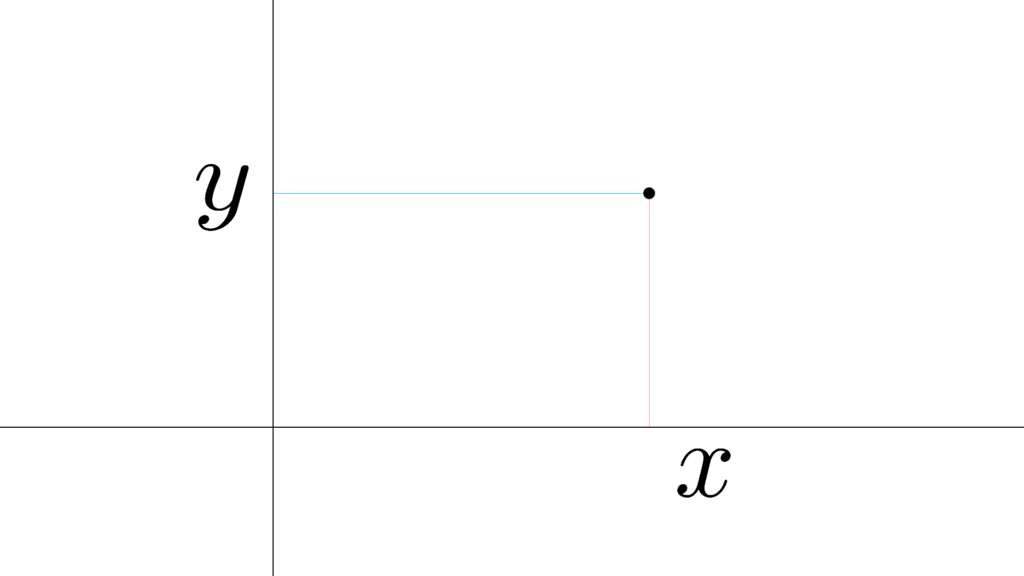
よく見る ↑ の画像のやつの名前は

「直交座標系（デカルト座標系）」です。

座標と座標系

「座標」は『点の位置を表現する数の組』のこと

$\begin{array}{llllll} \displaystyle (0,0) && (x,y) \end{array}$

「座標系」は『座標の意味を決めるもの』のことで

「原点・座標軸の取り方」といった

『図形を視覚化する』操作は

「座標系」が担当する役割になります。

直交座標系 Rectangular

|| 最も直感的な座標の決め方

「デカルト座標系」とも呼ばれます。

まあこれは説明不要でしょう。

「座標」って言ったらだいたいこれですし。

極座標系 Polar

|| よく使う座標系その２

「長さ $r$ 」と「角度 $θ$ 」で決める方法

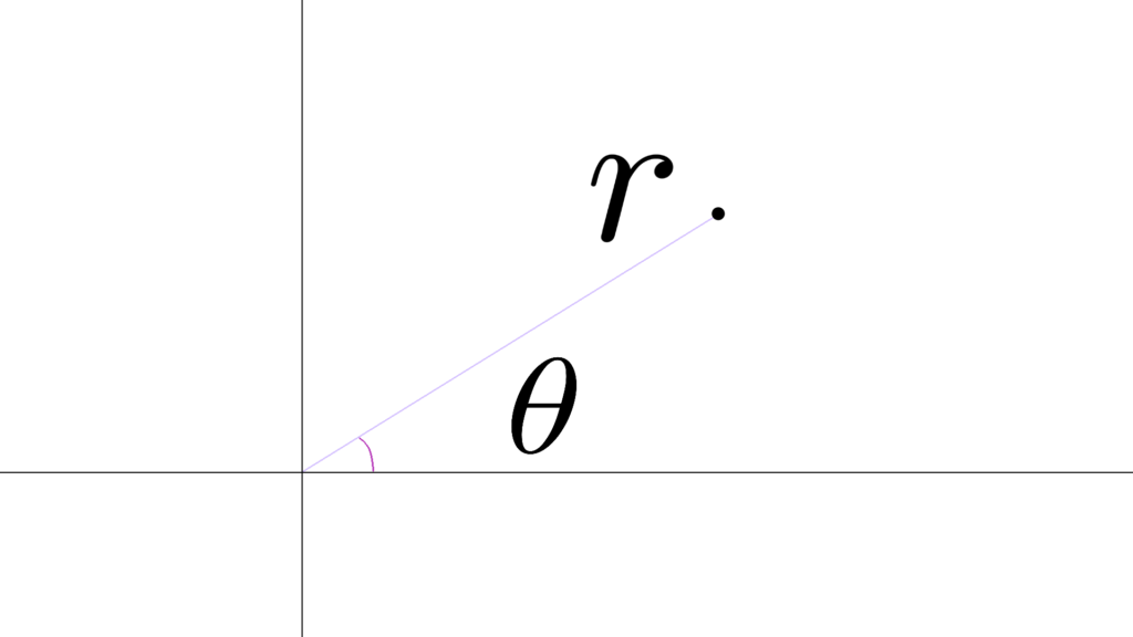
$\begin{array}{llllll} \displaystyle x&=&r\cos θ \\ \\ y&=&r\sin θ \end{array}$

$\begin{array}{llllll} \displaystyle r&=&\displaystyle \sqrt{x^2+y^2} \end{array}$

「複素平面」の話なんかで出てくるやつで

主に『回転』操作を行う時によく使われます。

空間での座標系

「空間（３次元）」でも

『直交座標系』は当然として

$(x,y,z)$

『極座標系』の考え方を使った

「円筒座標系（ $z$ だけ直交座標系）」ってやつと

$\begin{array}{llllll} \displaystyle x&=&r\cos θ \\ \\ y&=&r\sin θ \\ \\ z&=&z \end{array}$

「球面座標系（極座標系の拡張）」ってやつがあります。

$\begin{array}{llllll} \displaystyle x&=&r\cos θ\sin φ \\ \\ y&=&r\sin θ \sin φ \\ \\ z&=&r\cos φ \end{array}$

この辺りからちょっと複雑ですが

基本的な考え方は「平面」の話と同様ですね。

線形空間 Vector Space

|| ベクトルを問題なく使える保証

「線型空間」「ベクトル空間」とも呼ばれます。

$\begin{array}{cccccc} \displaystyle v,u,w&∈&V &&V \,\, \mathrm{is} \,\, \mathrm{Set \,\, of \,\, Vector} \\ \\ a,b&∈&S &&S \,\, \mathrm{is} \,\, \mathrm{Scalar \,\, Field} \end{array}$

$\begin{array}{cccccccc} \displaystyle (v+u)+w&=&v+(u+w) &&\mathrm{Associative} \\ \\ v+u&=&u+v &&\mathrm{Commutative} \\ \\ \\ v+\vec{0}&=&v&&\mathrm{Identity} \\ \\ v+(-v)&=&0 &&\mathrm{Inverse} \\ \\ \\ a\times (b\times v)&=&(a\times b)\times v&&\mathrm{Associative} \\ \\ 1\times v&=&v&&\mathrm{Identity} \\ \\ \\ a\times (v+u)&=&a\times v+a\times u&&\mathrm{Distributive} \\ \\ (a+b)\times v&=&a\times v+b\times v&&\mathrm{Distributive} \end{array}$

$\begin{array}{llllll} \displaystyle (V,+,\times) \,\, \mathrm{is} \,\, \mathrm{Vector \,\, Space} \,\, \mathrm{on} \,\, S \end{array}$

ざっくりとした定義はこんな感じですが

とりあえずこれは一端スルーでOK

ベクトル Vector

|| スカラー値を並べたやつ

「スカラーを拡張したもの」のこと

$\begin{array}{llllll} \displaystyle x,y &&→&&(1,2) \end{array}$

「方向を持つ点」「組み合せ・セット」といった

そういう感覚を形式的に表現したものになります。

実践的には

$\begin{array}{llllll} \displaystyle \mathrm{list} &=& [A,B,C,D,E,F] \end{array}$

「配列・行列」の形式でよく使われます。

求められる性質

これは以下のような

「持っていて欲しい性質」から

$\begin{array}{llllll} \displaystyle \vec{v}&=&(1,2) \\ \\ \vec{u}&=&(2,3) \end{array}$

矛盾が出ないよう定義されています。

$\begin{array}{cccccc} \vec{v}+\vec{u} &=& (3,5) && \mathrm{Addition} &\mathrm{Move} \\ \\ \displaystyle 2\vec{v} &=&(2,4) && \mathrm{Multiplication} & \mathrm{Length} \end{array}$

こういった性質は定義なんですが

順番は要請が先なので気を付けましょう。

座標系の変換

この「ベクトル」という概念を使うと

異なる２つの「座標系」があった時

$\begin{array}{llllll} \displaystyle \begin{array}{llllll} \textcolor{gray}{1,3} & 2,3 \\ \\ \displaystyle 1,2 & \textcolor{gray}{2,2} \end{array} &&\to&& \begin{array}{llllll} \displaystyle \textcolor{gray}{0,1} & 1,1 \\ \\ 0,0 & \textcolor{gray}{1,0} \end{array} &&-(1,2) \\ \\ \\ \begin{array}{llllll} \textcolor{gray}{0,\displaystyle\frac{1}{2}} & \displaystyle\frac{1}{2},\frac{1}{2} \\ \\ \displaystyle 0,0 & \displaystyle\textcolor{gray}{\frac{1}{2},0} \end{array} &&\to&& \begin{array}{llllll} \displaystyle \textcolor{gray}{0,1} & 1,1 \\ \\ 0,0 & \textcolor{gray}{1,0} \end{array}&&\times 2 \end{array}$

$\begin{array}{llllll} \displaystyle \begin{array}{llllll} \textcolor{gray}{0,\sin 45°} & \displaystyle\cos 45°,\sin 45° \\ \\ \displaystyle 0,0 & \textcolor{gray}{\cos 45°,0} \end{array} &&\to&& \begin{array}{llllll} \textcolor{gray}{0,\sin 60°} & \displaystyle\cos 60°,\sin 60° \\ \\ \displaystyle 0,0 & \textcolor{gray}{\cos 60°,0} \end{array} \end{array}$

「平行移動」「伸縮」「回転」

こういったことが理解しやすくなります。

ノルム Norm

|| 距離とか長さを拡張した概念

「ベクトル」の『長さ』を意味するもの

$\begin{array}{llllll} \displaystyle v_2&=&(x,y) \\ \\ v_3&=&(x,y,z) \end{array}$

$\begin{array}{llllll} \displaystyle ||v_2||_2&=&\displaystyle\sqrt{x^2+y^2} \\ \\ \displaystyle ||v_3||_2&=&\displaystyle\sqrt{x^2+y^2+z^2} \end{array}$

代表的なこれらは

「ユークリッドノルム」と呼ばれるもので

$\begin{array}{llllll} \displaystyle ||v_3||_2&=&\displaystyle \left( x^2+y^2+z^2 \right)^{\frac{1}{2}} \\ \\ \displaystyle ||v_3||_p&=&\displaystyle \left( x^p+y^p+z^p \right)^{\frac{1}{p}} \end{array}$

更に一般化されたものは

こんな感じの記号で表現されます。

ただまあ使うのはほぼ「 $2$ -ノルム」で

$\begin{array}{llllll} \displaystyle ||v||_2&≒&||v|| \end{array}$

「ノルム」って言ったら

だいたい「 $2$ -ノルム」のことを指します。

内積 Inner Product

|| ベクトルの掛け算的な操作

「異なるベクトル」のノルムを求める感じ。

$\begin{array}{llllll} \displaystyle v&=&(a,b,c) \\ \\ q&=&(x,y,z) \end{array}$

$\begin{array}{ccc} v \cdot q &=& \displaystyle ax+by+cz \\ \\ \langle v,q \rangle&=& \displaystyle ax+by+cz \end{array}$

「方向を合わせて掛ける」感じの操作とも言えます。

$\begin{array}{ccc} \displaystyle v \cdot u &=&||v|| \, ||u|| \, \cos θ \\ \\ \langle v,v \rangle &=&||v|| \, ||v|| \, \cos 0 &=&||v||^2\end{array}$

これの歴史はわりとぐちゃぐちゃなので

発生起源やらなんやらはよく分かりません。

（第一人者はハミルトン・テイト・グラスマン）

内積の感覚

これは以下の感覚を定式化したもので

（「線型」なんて呼ばれる感覚）

$\begin{array}{llllll} \displaystyle ax+by &→&(a,b)(x,y) \\ \\ ax+by+cz &→&(a,b,c)(x,y,z) \end{array}$

$\begin{array}{cccc} \displaystyle a_0 x^0 + a_1 x^1 + a_2 x^2 + \cdots + a_n x^n &=&0 \\ \\ x_1 p_1 + x_2 p_2 + x_3 p_3 + \cdots + x_np_n &=&E(X) \end{array}$

基本的にそれ以上の意味を持ちません。

良い感じのツールという側面が強いです。

四元数 Quaternion

物理学における「仕事」に始まり

「ベクトル」の基盤と言える概念は

$\begin{array}{llllll} \displaystyle q&=&a_0+a_1i+a_2j+a_3k \end{array}$

$\begin{array}{ccc} \displaystyle i^2&=& j^2&=& k^2&=& ijk&=&-1 \end{array}$

$\begin{array}{ccrrrrr} \displaystyle &&\times i&\times j&\times k \\ \\ i&& -1 & k & -j \\ \\ j&& -k & -1 & i \\ \\ k&& j & -i & -1 \end{array}$

$\begin{array}{ccr} \displaystyle 〇×&=&△ \\ \\ ×〇&=&-△ \end{array}$

『独立した回転』を可能にする

「四元数 $q$ 」と呼ばれてるものになります。

$\begin{array}{llllll} \displaystyle \overbrace{a_0}^{\mathrm{Scalar}}+\underbrace{a_1i+a_2j+a_3k}_{\mathrm{Vector}} \end{array}$

$\begin{array}{llllll} \displaystyle a_1i+a_2j+a_3k &⇆& (a_1,a_2,a_3) \end{array}$

数式としてはこんな感じで

$\begin{array}{llllll} vu&=& \displaystyle (a_1i+a_2j+a_3k)(b_1i+b_2j+b_3k) \end{array}$

$\begin{array}{llllll} \displaystyle \begin{array}{llllll} \displaystyle a_1ib_1i+a_1ib_2j+a_1ib_3k \\ \\ a_2jb_1i+a_2jb_2j+a_2jb_3k \\ \\ a_3kb_1i+a_3kb_2j+a_3kb_3k \end{array} &=&\displaystyle \begin{array}{r} \displaystyle -a_1b_1+a_1b_2ij+a_1b_3ik \\ \\ a_2b_1ji-a_2b_2+a_2b_3jk \\ \\ a_3b_1ki+a_3b_2kj-a_3b_3 \end{array} \end{array}$

$\begin{array}{r} \displaystyle \textcolor{pink}{-a_1b_1}+a_1b_2\textcolor{steelblue}{k}-a_1b_3\textcolor{mediumaquamarine}{j} \\ \\ -a_2b_1\textcolor{steelblue}{k}\textcolor{pink}{-a_2b_2}+a_2b_3\textcolor{greenyellow}{i} \\ \\ a_3b_1\textcolor{mediumaquamarine}{j}-a_3b_2\textcolor{greenyellow}{i}\textcolor{pink}{-a_3b_3} \end{array}$

$\begin{array}{r} \displaystyle -(a_1b_1+a_2b_2+a_3b_3) \\ \\ (a_2b_3-a_3b_2)\textcolor{greenyellow}{i} \\ \\ (a_3b_1-a_1b_3)\textcolor{mediumaquamarine}{j} \\ \\ (a_1b_2-a_2b_1)\textcolor{steelblue}{k} \end{array}$

ややこしいですが

「スカラー」部分と『その他』の部分から

$\begin{array}{cccccc} \displaystyle a_1b_1+a_2b_2+a_3b_3 &&\mathrm{Inner} && \mathrm{Scalar} \\ \\ \displaystyle \left( \begin{array}{llllll} \displaystyle a_2b_3-a_3b_2 \\ a_3b_1-a_1b_3 \\ a_1b_2-a_2b_1 \end{array} \right)&&\mathrm{Outer} && \mathrm{Vector} \end{array}$

結果的に

『ベクトル計算のスカラー部分』として

「内積」はこのような形で定義されました。

まとめると

つまり「内積」という操作は

$\begin{array}{llllll} \displaystyle v\cdot u&=&a_1b_1+a_2b_2+a_3b_3 \end{array}$

「ベクトル同士の掛け算」による

『スカラー値の抽出』を意味する操作だと言えます。

行列 Matrix

|| ベクトルを拡張したやつ

「ベクトル」の「ベクトル」みたいな感じ

$\begin{array}{ccccr} ax+by &&→&& \displaystyle \left( \begin{array}{llllll} \displaystyle a&b \end{array} \right) \displaystyle \left( \begin{array}{llllll} \displaystyle x \\ y \end{array} \right) \\ \\ \displaystyle \left( \begin{array}{llllll} \displaystyle ax+by \\ cx+dy \end{array} \right)&&→&& \displaystyle \left( \begin{array}{llllll} \displaystyle a&b \\ c&d \end{array} \right) \displaystyle \left( \begin{array}{llllll} \displaystyle x \\ y \end{array} \right) \end{array}$

$\begin{array}{llllll} \displaystyle \left( \begin{array}{llllll} \displaystyle ax+by&av+bu \\ cx+dy&cv+du \end{array} \right)&&→&& \displaystyle \left( \begin{array}{llllll} \displaystyle a&b \\ c&d \end{array} \right) \displaystyle \left( \begin{array}{llllll} \displaystyle x & v \\ y & u \end{array} \right) \end{array}$

$\begin{array}{llllll} \displaystyle \left( \begin{array}{llllll} \displaystyle \vec{a_1} \\ \vec{a_2} \end{array} \right)&=&\displaystyle \left( \begin{array}{llllll} \displaystyle a_{11}&a_{12} \\ a_{21} & a_{22} \end{array} \right) \end{array}$

「連立方程式」とか

$\begin{array}{rrr} \displaystyle \left( \begin{array}{llllll} \displaystyle 1&0&0 \\ 0&1&0 \\ 0&0&1 \end{array} \right) \displaystyle \left( \begin{array}{llllll} \displaystyle x \\ y \\ z \end{array} \right) &=&\displaystyle \left( \begin{array}{llllll} \displaystyle a \\ b \\ c \end{array} \right) \\ \\ \\ \displaystyle A^{-1}A\left( \begin{array}{llllll} \displaystyle x \\ y \\ z \end{array} \right) &=&\displaystyle A^{-1}\left( \begin{array}{llllll} \displaystyle c_1 \\ c_2 \\ c_3 \end{array} \right) \end{array}$

「配列（ベクトル）の一括処理」

「点座標の一括処理」なんかでよく見ます。

$\begin{array}{llllll} F(\mathrm{Data}_{\mathrm{matrix}}) &=& \displaystyle \left( \begin{array}{cccc} \displaystyle F(\mathrm{Data}_{\mathrm{vector}}) \\ \\ F(\mathrm{Data}_{\mathrm{vector}}) \\ \\ F(\mathrm{Data}_{\mathrm{vector}}) \\ \\ \vdots \end{array} \right) \end{array}$

「画像の処理」とかが実感しやすいかもしれません。

身近な活用事例

こいつは一見するとよくわからんですが

実は身近なものにわりと使われていて

$\begin{array}{llllll} \displaystyle \left( \begin{array}{llllll} [255,0,0]&[0,255,0]&[0,0,255] \\ \\ [255,255,0]&[0,255,255] & [255,0,255] \\ \\ [0,0,0]&[127,127,127]&[255,255,255] \end{array} \right) \end{array}$

例えば「画像のRGB」なんかをまとめて

「平行移動・伸縮・回転」なんかの

一括処理を行う場合とかで使われてます。

単位行列 Identity Matrix

「行列」の「かけ算的な操作」

（正方行列の話になります）

$\begin{array}{rclcc} IA&=&AI&=&A \\ \\ \displaystyle EA&=&AE&=&A \\ \\ \hat{1}A&=& A\hat{1}&=&A \end{array}$

$\begin{array}{llllll} \displaystyle I_2&=&\displaystyle \left( \begin{array}{ccc} \displaystyle 1&0 \\ 0&1 \end{array} \right) \\ \\ \mathrm{diag}(1,1)&=&\displaystyle \left( \begin{array}{ccc} \displaystyle 1&0 \\ 0&1 \end{array} \right) \end{array}$

これによって

「変化を起こさない行列」のことを

「単位行列」と言って

$\begin{array}{llllll} \displaystyle \left( \begin{array}{ccc} \displaystyle a&b \\ c&d \end{array} \right)\displaystyle \left( \begin{array}{ccc} \displaystyle 1&0 \\ 0&1 \end{array} \right)&=&\displaystyle \left( \begin{array}{ccc} \displaystyle a&b \\ c&d \end{array} \right) \end{array}$

具体的にはこういうやつが単位行列になります。

逆行列 Inverse Matrix

ある行列を「単位行列にする行列」のこと。

（掛け算で言うところの逆数みたいなやつ）

$\begin{array}{llllll} \displaystyle AA^{-1}&=&I \end{array}$

$\begin{array}{llllll} \displaystyle A^{-1} &=& \displaystyle \frac{1}{\mathrm{det}(A)}\left( \begin{array}{ccc} \displaystyle d&-b \\ -c&a \end{array} \right) \end{array}$

導出は力技です。

$\begin{array}{llllll} \displaystyle \left( \begin{array}{ccc} \displaystyle a&b \\ c&d \end{array} \right)A^{-1} &=& \displaystyle \left( \begin{array}{ccc} \displaystyle 1&0 \\ 0&1 \end{array} \right) \end{array}$

これから得られる連立方程式を解くと

$\begin{array}{llllll} \displaystyle \left( \begin{array}{ccc} \displaystyle a&b \\ c&d \end{array} \right)\left( \begin{array}{ccc} \displaystyle x_{11}&x_{12} \\ x_{21}&x_{22} \end{array} \right) &=& \displaystyle \left( \begin{array}{ccc} \displaystyle ax_{11}+bx_{21}&ax_{12}+bx_{22} \\ cx_{11}+dx_{21}&cx_{12}+dx_{22} \end{array} \right) \end{array}$

$\begin{array}{llllll} \displaystyle \left\{ \begin{array}{llllll} \displaystyle ax_{11}+bx_{21}&=&1 \\ cx_{11}+dx_{21}&=&0 \end{array} \right. &&\to&& \displaystyle \left\{ \begin{array}{llllll} \displaystyle acx_{11}+bcx_{21}&=&c \\ acx_{11}+adx_{21}&=&0 \end{array} \right. \\ \\ \\ \displaystyle \left\{ \begin{array}{llllll} \displaystyle ax_{12}+bx_{22}&=&0 \\ cx_{12}+dx_{22}&=&1 \end{array} \right. &&\to&& \displaystyle \left\{ \begin{array}{llllll} \displaystyle acx_{12}+bcx_{22}&=&0 \\ acx_{12}+adx_{22}&=&a \end{array} \right. \end{array}$

$\begin{array}{llllll} (ad-bc)x_{21}&=&-c &&\to&&cx_{11}+dx_{21}&=&0 \\ \\ (ad-bc)x_{22}&=&a &&\to&& ax_{12}+bx_{22}&=&0 \end{array}$

$\begin{array}{llllll} \displaystyle \left( \begin{array}{ccc} \displaystyle x_{11}&x_{12} \\ x_{21}&x_{22} \end{array} \right) &=&\displaystyle \frac{1}{ad-bc}\left( \begin{array}{ccc} \displaystyle d&-b \\ -c&a \end{array} \right) \end{array}$

$\begin{array}{ccccc} \displaystyle A^{-1}A&=&I &&？ \\ \\ A^{-1}I&=&A^{-1} &&〇 \\ \\ A^{-1}AA^{-1}&=&A^{-1} &&〇 \\ \\ (A^{-1}A)A^{-1}&=&A^{-1} &&〇 \end{array}$

$\begin{array}{llllll} \displaystyle AA^{-1}&=&I&=&A^{-1}A \end{array}$

この結果に行き着きます。

またこれに伴い

$\begin{array}{cccccc} \displaystyle ad-bc&=& 0 &&\mathrm{No} \\ \\ ad-bc&≠&0 && \mathrm{Exist} \end{array}$

この値から

「逆行列の存在」を判定できるようになります。

線形写像 Linear Mapping

|| 点をどこにでも移動させることができる

「点を動かす」ことになる「行列」の名前

$\begin{array}{llllll} \displaystyle A \left( \begin{array}{llllll} \displaystyle x \\ y \end{array} \right)&=&\left( \begin{array}{llllll} \displaystyle x_A \\ y_A \end{array} \right) \end{array}$

「線型変換」「一次変換」とも呼ばれます。

あまり直感的には理解しにくいですが

「連立方程式」の感覚から分かる通り

$\begin{array}{llllll} \displaystyle \left( \begin{array}{llllll} \displaystyle a&b \\ c&d \end{array} \right) \displaystyle \left( \begin{array}{llllll} \displaystyle x \\ y \end{array} \right) &=&\displaystyle \left( \begin{array}{llllll} \displaystyle α \\ β \end{array} \right) \end{array}$

『連立方程式の係数』をまとめた「行列」

この中身 $a,b,c,d$ を好きに書き換えれば

$\begin{array}{llllll} \displaystyle \left( \begin{array}{llllll} \displaystyle x \\ y \end{array} \right) &→&\displaystyle \left( \begin{array}{llllll} \displaystyle α \\ β \end{array} \right) \end{array}$

『あらゆる場所』に点を移動させることができる

というのはなんとなく実感できると思います。

$\begin{array}{llllll} \displaystyle \left( \begin{array}{llllll} \displaystyle a&b \\ c&d \end{array} \right) \displaystyle \left( \begin{array}{llllll} \displaystyle 0 \\ 0 \end{array} \right) &=&\displaystyle \left( \begin{array}{llllll} \displaystyle 0 \\ 0 \end{array} \right) \end{array}$

同様に

これが「原点 $(0,0)$ を動かさない」

ということも分かるかと。

伸縮

分かりやすい話

$\begin{array}{llllll} 2I &=& \displaystyle \left( \begin{array}{llllll} \displaystyle 2&0 \\ 0&2 \end{array} \right) \end{array}$

例えば「定数倍した単位行列」は

$\begin{array}{llllll} \displaystyle \left( \begin{array}{llllll} \displaystyle 2&0 \\ 0&2 \end{array} \right) \displaystyle \left( \begin{array}{llllll} \displaystyle x \\ y \end{array} \right) &=&\displaystyle \left( \begin{array}{llllll} \displaystyle 2x \\ 2y \end{array} \right) \end{array}$

「伸縮させる線型写像」です。

これは直感的に分かると思います。

回転行列 Rotate

「極座標系」の感覚から

$\begin{array}{lcrlllll} \displaystyle x&=&r\cos α \\ y&=&r\sin α \end{array}$

$\begin{array}{lcc} \displaystyle R_{θ} \displaystyle \left( \begin{array}{r} \displaystyle r\cos α \\ r\sin α \end{array} \right) &=&\displaystyle \left( \begin{array}{r} \displaystyle r\cos (θ+α) \\ r\sin (θ+α) \end{array} \right) \end{array}$

「三角関数の加法定理」より

$\begin{array}{rr} \displaystyle \cos (θ+α)&=&\cos θ\cos α - \sin θ \sin α \\ \sin (θ+α)&=&\sinθ \cos α + \cosθ \sin α \end{array}$

$\begin{array}{llllll} \displaystyle \left( \begin{array}{r} \displaystyle \cos (θ+α) \\ \sin (θ+α) \end{array} \right) &=& \displaystyle \left( \begin{array}{rr} \displaystyle \cos θ & -\sin θ \\ \sin θ & \cos θ \end{array} \right) \left( \begin{array}{rr} \displaystyle \cos α \\ \sin α \end{array} \right) \end{array}$

以下のような

$\begin{array}{llllll} \displaystyle R_θ&=&\displaystyle \left( \begin{array}{rr} \displaystyle \cos θ & -\sin θ \\ \sin θ & \cos θ \end{array} \right) \end{array}$

『その場から $θ$ 回転させる』ことになる

「線型写像」を得ることができます。

ちなみに

$\begin{array}{llllll} \displaystyle \left( \begin{array}{llllll} \displaystyle 1&0 \\ 0&1 \end{array} \right) &=&\displaystyle \left( \begin{array}{rr} \displaystyle \cos 0 & -\sin 0 \\ \sin 0 & \cos 0 \end{array} \right) \end{array}$

「回転行列」の視点から見ると

「単位行列」は「回転させない操作」になります。

任意の位置に移動させられる

以上の話から分かると思いますが

$\begin{array}{llllll} \displaystyle tIR_θ&=&\displaystyle \left( \begin{array}{llllll} \displaystyle t&0 \\ 0&t \end{array} \right)\left( \begin{array}{rr} \displaystyle \cos θ & -\sin θ \\ \sin θ & \cos θ \end{array} \right) \end{array}$

「極座標系」を知っていれば分かる通り

この２つの「線形写像」があれば

$\begin{array}{llllll} \displaystyle \left( \begin{array}{llllll} \displaystyle t&0 \\ 0&t \end{array} \right) \left( \begin{array}{rr} \displaystyle \cos θ & -\sin θ \\ \sin θ & \cos θ \end{array} \right) \left( \begin{array}{rr} \displaystyle r\cos α \\ r\sin α \end{array} \right) &=& \displaystyle \left( \begin{array}{r} \displaystyle tr\cos (θ+α) \\ tr\sin (θ+α) \end{array} \right) \end{array}$

「原点以外の点」であれば

あらゆる座標に移動させることが可能になります。

これは『 $(1,0)$ に変換できる』という事実から

$\begin{array}{llllll} \displaystyle \frac{1}{r} \left( \begin{array}{rr} \displaystyle \cos (-α) & -\sin (-α) \\ \sin (-α) & \cos (-α) \end{array} \right) \left( \begin{array}{rr} \displaystyle r\cos α \\ r\sin α \end{array} \right) &=&\displaystyle \left( \begin{array}{rr} \displaystyle \cos 0 \\ \sin 0 \end{array} \right) \end{array}$

直感的に理解できるかと。

行列式 Determinant

|| 正方行列で定義できる意味のある量

「逆行列」から導かれるやつ

$\begin{array}{lcc} A&=&\displaystyle \left( \begin{array}{ccc} \displaystyle a&b \\ c&d \end{array} \right) \\ \\ A^{-1} &=& \displaystyle \frac{1}{\mathrm{det}(A)}\left( \begin{array}{ccc} \displaystyle d&-b \\ -c&a \end{array} \right) \end{array}$

$\begin{array}{ccc} \displaystyle \mathrm{det}(A)&=&\displaystyle \left| \begin{array}{ccc} \displaystyle a&b \\ c&d \end{array} \right| \\ \\ &=&ad-bc \end{array}$

この時点じゃこれだけの意味しか持ちません。

行列式と面積

「面積 $1$ の正方形」を

『線型写像（行列）で拡大する』

そういった操作を考えた時の

$\begin{array}{llllll} \displaystyle I&=&\displaystyle \left( \begin{array}{ccc} \displaystyle 1&0 \\ 0&1 \end{array} \right) \end{array}$

「正方形」を変形する

「線形写像としての行列 $A$ 」

その演算結果から作られる「平行四辺形」

$\begin{array}{llllll} A&=&\displaystyle \left( \begin{array}{ccc} \displaystyle a&b \\ c&d \end{array} \right) \end{array}$

$\begin{array}{llllll} \displaystyle A \left( \begin{array}{ccc} \displaystyle 1 \\ 0 \end{array} \right)&=&\displaystyle \left( \begin{array}{ccc} \displaystyle a \\ c \end{array} \right) \\ \\ \displaystyle A \left( \begin{array}{ccc} \displaystyle 0 \\ 1 \end{array} \right)&=&\displaystyle \left( \begin{array}{ccc} \displaystyle b \\ d \end{array} \right) \end{array}$

（正方形を成す単位ベクトル $(1,0),(0,1)$ の移動）

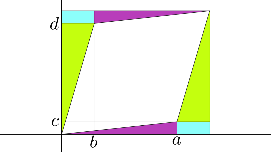
$\begin{array}{llllll} \displaystyle (a+b)(c+d)&=&\textcolor{darkmagenta}{ac}+ad+\textcolor{aqua}{bc}+\textcolor{greenyellow}{bd} \end{array}$

$\begin{array}{rcc} \displaystyle \textcolor{aqua}{bc}×2 \\ \\ \displaystyle \frac{1}{2} \textcolor{darkmagenta}{ac}×2 \\ \\ \displaystyle \frac{1}{2} \textcolor{greenyellow}{db}×2 \end{array}$

$\begin{array}{llllll} \displaystyle (a+b)(c+d) - \left( 2\textcolor{aqua}{bc}+\frac{1}{2} 2\textcolor{darkmagenta}{ac} + \frac{1}{2} 2\textcolor{greenyellow}{db} \right) &=&ad-bc \\ \\ &=&\mathrm{det}(A) \end{array}$

この面積もまた $\mathrm{det}(A)$ になります。

関数行列 Jacobian Matrix

|| ある関数の各変数の方向微分を並べた行列

『全微分の中身』を集めた「行列」のこと

$\begin{array}{llllll} \displaystyle |J|&=& \displaystyle\frac{\partial (x,y)}{\partial (r,θ)} &=&\displaystyle\frac{dxdy}{drdθ} \\ \\ && \displaystyle\frac{\partial (x,y)}{\partial (r,θ)} &=&\displaystyle\left| \begin{array}{llllll} \displaystyle \frac{\partial x}{\partial r} &\displaystyle\frac{\partial x}{\partial θ} \\ \\ \displaystyle\frac{\partial y}{\partial r} &\displaystyle\frac{\partial y}{\partial θ} \end{array} \right| \end{array}$

$\begin{array}{llllll} \displaystyle J&=&\displaystyle\left( \begin{array}{llllll} \displaystyle \frac{\partial x}{\partial r} &\displaystyle\frac{\partial x}{\partial θ} \\ \\ \displaystyle\frac{\partial y}{\partial r} &\displaystyle\frac{\partial y}{\partial θ} \end{array} \right) \end{array}$

「ヤコビ行列」「ヤコビアン」とも言われます。

$\begin{array}{ccc} \displaystyle x&=&(x_1,x_2,x_3,\cdots,x_i) \\ \\ f(x)&=&\displaystyle \left( \begin{array}{c} \displaystyle f_1(x_1,x_2,x_3,\cdots,x_i) \\ \\ f_2(x_1,x_2,x_3,\cdots,x_i) \\ \\ \vdots \\ \\ f_n(x_1,x_2,x_3,\cdots,x_i) \end{array} \right) \end{array}$

$\begin{array}{cccccccc} \displaystyle \displaystyle J_f&=&\displaystyle\left( \begin{array}{cccccccccccc} \displaystyle \frac{\partial f_1}{\partial x_1} & \displaystyle \frac{\partial f_1}{\partial x_2} &\cdots &\displaystyle\frac{\partial f_1}{\partial x_i} \\ \\ \vdots &\vdots &&\vdots \\ \\ \displaystyle\frac{\partial f_n}{\partial x_1} &\displaystyle\frac{\partial f_n}{\partial x_2} &\cdots &\displaystyle\frac{\partial f_n}{\partial x_i} \end{array} \right) \end{array}$

一般化するとこんな感じなんですが

これじゃなんも分からんですね。

ふわっとした意味

これはいったいなんなのか

簡単に説明するのは難しいですが

なんとなく

「まとめたもの」であることは分かると思います。

というのも

例えば「多変数関数の全微分」を行う場合

$\begin{array}{llllll} \displaystyle dz&=&df(x,y) \\ \\ &=&f(x+dx,y+dy)-f(x,y) \\ \\ &=&\displaystyle\frac{\partial f}{\partial x}dx +\frac{\partial f}{\partial y}dy \end{array}$

「座標 $z$ 」の計算から

「 $dz$ の微小変化」については

このように書かれるわけですが

これを分解して並べると

$\begin{array}{llllll} dz&=& \displaystyle \left( \begin{array}{llllll} \displaystyle \frac{\partial f}{\partial x} &\displaystyle \frac{\partial f}{\partial y} \end{array} \right) \left(\begin{array}{llllll} \displaystyle dx \\ dy \end{array}\right) \end{array}$

「内積」の形を考えれば

こんな感じになりますよね。

で、他の $x,y$ を変数に持つ関数 $g(x,y)$ を考えると

$\begin{array}{llllll} dz &=& \displaystyle \left( \begin{array}{llllll} \displaystyle \frac{\partial g}{\partial x} &\displaystyle \frac{\partial g}{\partial y} \end{array} \right) \left(\begin{array}{llllll} \displaystyle dx \\ dy \end{array}\right) \end{array}$

これもこうで

$\begin{array}{llllll} \displaystyle \left( \begin{array}{llllll} \displaystyle\frac{\partial f}{\partial x} &\displaystyle \frac{\partial f}{\partial y} \\ \\ \displaystyle \frac{\partial g}{\partial x} &\displaystyle \frac{\partial g}{\partial y} \end{array} \right) \left(\begin{array}{llllll} \displaystyle dx \\ dy \end{array}\right) \end{array}$

これらは「行列」の定義から

このように書くことができます。

$\begin{array}{llllll} \displaystyle \left( \begin{array}{llllll} \displaystyle\frac{\partial f}{\partial x}dx + \displaystyle \frac{\partial f}{\partial y}dy \\ \\ \displaystyle \frac{\partial g}{\partial x}dx + \displaystyle \frac{\partial g}{\partial y}dy \end{array} \right) \end{array}$

これは計算するとこうなりますから。

とまあ要はそんな感じで

$\begin{array}{llllll} \displaystyle dz&=&\displaystyle \left( \begin{array}{llllll} \displaystyle\frac{\partial f}{\partial x}dx + \displaystyle \frac{\partial f}{\partial y}dy \\ \\ \displaystyle \frac{\partial g}{\partial x}dx + \displaystyle \frac{\partial g}{\partial y}dy \end{array} \right) \end{array}$

「内積」で「全微分」を表現して拡張したもの

全ての偏微分の成分を綺麗に並べて整理したもの

$\begin{array}{llllll} \displaystyle J&=&\displaystyle\left( \begin{array}{llllll} \displaystyle \frac{\partial f}{\partial x} &\displaystyle\frac{\partial f}{\partial y} \\ \\ \displaystyle\frac{\partial g}{\partial x} &\displaystyle\frac{\partial g}{\partial y} \end{array} \right) \end{array}$

この辺りが

「関数行列」の持つ意味になります。

使用される例

これは主に「変数の変換」で用いられます。

$\begin{array}{llllll} \displaystyle x,y &&→&& r,θ \end{array}$

具体的には

「極座標系」への変換を行う時の

「微小面積・体積」の比率を求める時に

$\begin{array}{llllll} \displaystyle dxdy &&→&& drdθ \end{array}$

「行列式」から

「微小面積」を直接的に求めて

$\begin{array}{llllll} \displaystyle dxdy&=&\displaystyle\left| \begin{array}{llllll} \displaystyle \frac{\partial x}{\partial r} &\displaystyle\frac{\partial x}{\partial θ} \\ \\ \displaystyle\frac{\partial y}{\partial r} &\displaystyle\frac{\partial y}{\partial θ} \end{array} \right|drdθ \end{array}$

「座標系」間の変数の比率を求める、という感じで。

（この行列式もヤコビアンと呼ばれます）

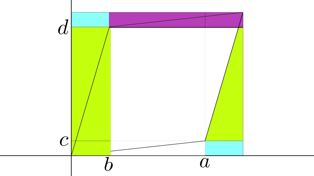
微小面積の導出

↑ の説明だけじゃ分からないと思うので

ちょっとこの辺りを補足しておくと

$\begin{array}{llllll} \displaystyle dxdy \end{array}$

まずやってることなんですが

これは「面積の計算」です。

$\begin{array}{llllll} 0,dy&&dx,dy \\ \\ \displaystyle 0,0 && 0,dx \end{array}$

これを「図形的に」見て

そのまま直接的に求める。

$\begin{array}{llllll} 底辺×高さ &&→&& \displaystyle dxdy \end{array}$

やってることはただそれだけで

$\begin{array}{llllll} \displaystyle dx&=& \displaystyle \frac{\partial x}{\partial r}dr +\displaystyle\frac{\partial x}{\partial θ}dθ \\ \\ dy&=&\displaystyle\frac{\partial y}{\partial r}dr +\displaystyle\frac{\partial y}{\partial θ}dθ \end{array}$

後はこの「全微分」の関係から

$\begin{array}{llllll} \displaystyle\left( \begin{array}{llllll} \displaystyle \frac{\partial x}{\partial r} &\displaystyle\frac{\partial x}{\partial θ} \\ \\ \displaystyle\frac{\partial y}{\partial r} &\displaystyle\frac{\partial y}{\partial θ} \end{array} \right) \displaystyle\left( \begin{array}{llllll} dr \\ dθ \end{array} \right) \end{array}$

「ヤコビアン」を「線型写像」とみなして

$\begin{array}{llllll} \begin{array}{llllll} \displaystyle\left( \begin{array}{llllll} \displaystyle \frac{\partial x}{\partial r} &\displaystyle\frac{\partial x}{\partial θ} \\ \\ \displaystyle\frac{\partial y}{\partial r} &\displaystyle\frac{\partial y}{\partial θ} \end{array} \right) \displaystyle\left( \begin{array}{llllll} dr \\ dθ \end{array} \right) \end{array}&=&\displaystyle\begin{array}{llllll} \displaystyle\left( \begin{array}{llllll} 1&0 \\ 0&1 \end{array} \right) \displaystyle\left( \begin{array}{llllll} dx \\ dy \end{array} \right) \end{array} \end{array}$

これらの面積を考えると

$\begin{array}{llllll}\displaystyle\left| \begin{array}{llllll} \displaystyle \frac{\partial x}{\partial r} &\displaystyle\frac{\partial x}{\partial θ} \\ \\ \displaystyle\frac{\partial y}{\partial r} &\displaystyle\frac{\partial y}{\partial θ} \end{array} \right| drdθ&=&\displaystyle\left| \begin{array}{llllll} 1&0 \\ 0&1 \end{array} \right| dxdy \end{array}$

↑ の等式からそのまま値を取り出せば

結果としてこのような結論が得られます。

目次